Getting Started
This tutorial provides an introduction to the basic use of Macroeco for ecological pattern analysis.
The functionality of the software Macroeco can be accessed through two interfaces: the low-level Python package macroeco or the high-level MacroecoDesktop interface.
The Python package macroeco is a scientific Python package that can be imported into a user’s custom scripts and modules along with other scientific packages such as scipy or pandas.
The MacroecoDesktop interface is designed for users who wish to use the functionality of Macroeco but are not Python programmers. Instead of writing Python code, users of MacroecoDesktop create simple text files, known as parameters files, that describe an analysis and the type of desired output. MacroecoDesktop provides both a window-based graphical interface and a “headless” command line mode - the latter of these allows MacroecoDesktop to be called from other computing environments such as R.
Installation
macroeco is written in Python 2.7. Users with an existing scientific Python environment that includes recent versions of numpy, scipy, pandas, matplotlib, and wxpython can install macroeco from the Python Package Index (PyPI) using the command pip install macroeco. Additional dependencies will be installed automatically as necessary.
For users wishing to install a new scientific Python environment, we recommend installing the Anaconda or Miniconda Python 2.7 distribution (64-bit) from Continuum Analytics (http://continuum.io/). While larger in size, the Anaconda installer contains a complete scientific Python ecosystem and is packaged with an easy-to-use graphical installer. During installation, select the option to add Anaconda to the system path environment variable.
After installing either Anaconda or Miniconda, close and reopen a terminal window, then type the command which python (where python on Windows) and ensure that the path that is returned contains the word anaconda or miniconda. Then run the command conda install numpy scipy pandas matplotlib wxpython pip followed by the command pip install macroeco, to complete the installation of macroeco.
An optional dependency shapely is needed for the analysis of spatial beta diversity patterns. As this package depends on the GEOS framework, it must be installed manually. Users wishing to install shapely should refer to the package documentation for more details.
As an alternative to installing a Python environment, Mac OS X users who wish to use only MacroecoDesktop may instead download a standalone executable. This application allows users to perform MacroecoDesktop analyses through a graphical interface or from the command line, but does not support direct access to the lower-level functions in macroeco.
Users encountering difficulties when installing or running macroeco are invited to file an issue to request support.
The remainder of this tutorial uses demo data from a vegetation census in Anza-Borrego Desert State Park in southern California. This demo data can be downloaded at this link. The file ANBO.csv contains the census data and the file ANBO.txt contains metadata describing the data table. This data may be freely shared and used for analysis so long as credit is given to the authors.
First steps: macroeco
Users of MacroecoDesktop should skip this section and proceed below to First steps: MacroecoDesktop.
The macroeco package contains three main subpackages of interest:
- Empirical - loads data tables and performs empirical analysis of macroecological metrics, such as the species abundance distribution and species area relationship
- Models - provides objects for distributions and curves predicted by macroecological theory, such as the logseries distributions and power law function
- Compare - provides utility functions for comparing the fit of models to empirical metrics, such as AIC weights and r-squared statistics
A common workflow involves loading data, calculating an empirical metric, fitting one or more models to the empirical metric, and evaluating the fit of the model to the metric. The following example calculates a simple species abundance distribution for the demo data.
First, the Patch class from the empirical subpackage is used to create a Patch object that holds the data table and a metadata dictionary describing the data. Patch requires a path, absolute or relative, to a metadata file as a mandatory argument (see Preparing Data for information on creating a metadata file for a new data set).
>>> import macroeco as meco
>>> pat = meco.empirical.Patch('~/Desktop/demo/ANBO.txt')
The empirical subpackage contains a number of functions that operate on patch objects and return macroecological metrics. Here we’ll use the function sad to calculate a species abundance distribution. The first argument is the patch object to use, the second is a string specifying which column has the species names (spp_col) and which, if any, has a count of individuals at a particular location (count_col), and the third is a string specifying how to split the data (see the Reference guide for the functions in the empirical module for more information on input arguments).
>>> sad = meco.empirical.sad(pat, 'spp_col:spp; count_col:count', '')
All functions for macroecological metrics return their results as a list of tuples. Each tuple has two elements: a string describing how the data were split and a result table with a column y (for univariate distributions like the species abundance distribution) or columns y and x (for curves such as a species area relationship) giving the results of the analysis. Since the data were not split in this example, the list has only one tuple.
Any number of distributions from the models subpackage can be fit to the resulting empirical metric. The code below fits the two parameters of the LINK upper truncated logseries distribution and uses the function AIC from the compare subpackage to calculate the AIC for this distribution and data.
>>> p, b = meco.models.logser_uptrunc.fit_mle(sad[0][1]['y'])
>>> p, b
(0.9985394369365049, 2445.0)
>>> meco.compare.AIC(sad[0][1]['y'], meco.models.logser_uptrunc(p, b))
208.61902087378027
The two fitted parameters can be used to generate a rank abundance distribution of the same length as the empirical data. The empirical and predicted rank curves are plotted.
>>> import numpy as np
>>> import matplotlib.pyplot as plt
>>> plt.semilogy(meco.models.logser_uptrunc.rank(len(sad[0][1]),p,b)[::-1])
>>> plt.semilogy(np.sort(sad[0][1]['y'])[::-1])
>>> plt.show()
For information on performing more complex analyses using macroeco, see Using macroeco.
First steps: MacroecoDesktop
This section describes the MacroecoDesktop interface. The purpose of MacroecoDesktop is to provide non-programmers an interface for accessing the functionality of Macroeco without the need to write Python code. Instead, the user creates a text file, called a parameters file, that contains the information and instructions needed by MacroecoDesktop to execute an analysis.
This section gives a very brief overview of how to create a simple parameter file and use it to analyze a species abundance distribution (the analysis and output are identical to that shown above in First steps: macroeco). More information on the structure of parameter files and how to customize them can be found in the tutorial MacroecoDesktop Recipes.
A parameter file can be created using the graphical interface included with MacroecoDesktop or using a plain text editor.
Users who wish to use the graphical interface and who have installed the macroeco package can open the graphical window by running the command python -c "import macroeco; macroeco.desktop()" at the command line (Mac users may need to replace python with pythonw). Mac OS X users who have downloaded the standalone MacroecoDesktop executable can instead simply double click on the application.
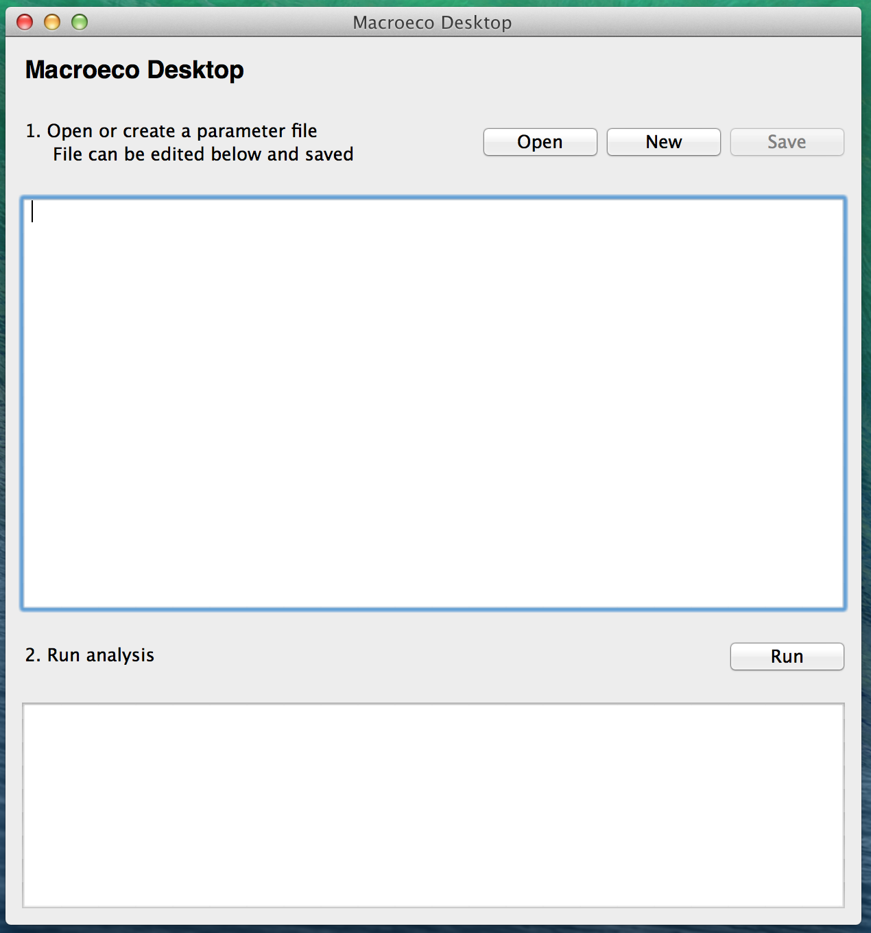
In the window shown above, a user first clicks the New button and chooses a name and location for the parameter file. The user then enters text into the top text box and uses the Save button to save this information as a parameter file. Previously created parameter files can be opened with the Open button.
Users who wish to create the parameter file using a text editor should instead create and save a plain text file containing all relevant parameters, as described below.
For our sample analysis, type the following text into your text editor. Save this file with the name new_parameters.txt in the demo directory containing the ANBO.txt and ANBO.csv files.
[SAD-ANBO]

analysis = sad

metadata = ANBO.txt

models = logser_uptrunc; lognorm
log_y = True
A single parameter file can contain multiple “runs”, each of which is denoted by the name of the run written in brackets (this run is titled SAD ANBO, as it will analyze the species abundance distribution for the Anza-Borrego demo data).
Conceptually, the information required for a single run can be broken down into three parts. The first part tells MacroecoDesktop the type of analysis that’s desired, in this case a species abundance distribution (any function contained in the empirical or models subpackage of macroeco can be listed here as an analysis).
The second part contains the information that MacroecoDesktop needs to complete the core analysis. To generate an empirical species abundance distribution, the necessary inputs are the location of a metadata file that both points to a data table and provides information about the data and a variable called “cols” that tells MacroecoDesktop which column in the data table represents the name of the species and which (if any) gives the count of individuals at a location.
The third part describes what, if any, theoretical models should be compared to the core empirical result and what options should be used for the comparison. The models variable gives a list of distribution names to compare to the empirical data. An additional variable log_y specifies that the y-axis of output graphs should be log transformed.
Once the parameter file has been created and saved, the MacroecoDesktop analysis can be started either from the graphical MacroecoDesktop program or from the Terminal.
From the graphical window, the user simply clicks the Save and Run button, and the bottom progress box will display real time output as the analysis runs. If the analysis encounters an error, it will be displayed here as well. When the analysis is complete, this box will report “Finished analysis successfully”.
From the command line, a user with a complete installation of macroeco can run the analysis using the command python -c "import macroeco; macroeco.desktop('\path\to\parameterfile').
For information on performing more complex analyses using MacroecoDesktop, see Using MacroecoDesktop.
First steps: Interpreting output
All the results generated from the parameter file new_parameters.txt are stored in a folder named results. In general the results folder will contain a log file (_log.txt) as well some number of folders. Each folder corresponds to a particular run specified in the parameters file.
In the case of the analysis that we ran above the log file should be similar to the output you saw on the MacroecoDesktop GUI or the terminal window
[2015/09/02 15:21:47 PM] {meco} INFO Running macroeco
[2015/09/02 15:21:47 PM] {meco} INFO Parameters file at /Users/mqwilber/Desktop/new_parameters.txt
[2015/09/02 15:21:47 PM] {meco} INFO Starting analysis
[2015/09/02 15:21:47 PM] {meco} INFO Starting run SAD-ANBO
[2015/09/02 15:21:47 PM] {meco} INFO Starting sad
[2015/09/02 15:21:47 PM] {meco} INFO Finished sad
[2015/09/02 15:21:47 PM] {meco} INFO Fitting models
[2015/09/02 15:21:47 PM] {meco} INFO Saving all results
[2015/09/02 15:21:48 PM] {meco} INFO Finished run SAD-ANBO
[2015/09/02 15:21:48 PM] {meco} INFO Finished analysis successfully
[2015/09/02 15:21:48 PM] {meco} INFO Results available at /Users/mqwilber/Desktop
The other folder in results should be named SAD-ANBO and it contains the results of the SAD-ANBO run specified in the new_parameters.txt file.
This folder contains 6 files
_subset_index.csv: This file contains a DataFrame specifying the different splits performed in the analysis. In this analysis, the ANBO data were not split in any way so the resulting csv file looks like
subsets 1
Where the 1 corresponds to the first split (which is blank) for this analysis. For information on splits see Empirical (macroeco.empirical) or A more complex analysis.
1_core_result.csv: This file contains the core result of the analysis for split 1. Because the file new_parameter.txt specified analysis = sad the core result is a species abundance distribution. spp gives the name of a species and y gives the abundance of that species.
spp y arsp1 2.0000 cabr 31.0000 caspi1 58.0000 chst 1.0000 comp1 5.0000 cran 4.0000 crcr 65.0000 crsp2 79.0000 enfa 1.0000 gnwe 41.0000 . . 1_data_models.csv: This file contains a comparison of the empirical species abundance distribution with the models specified in new_parameters.txt for the split 1. In this case models = logser_uptrunc; lognorm.
| x | spp | empirical | logser_uptrunc | logser_uptrunc_residual | lognorm | lognorm_residual |
|---|---|---|---|---|---|---|
| 24 | lesp1 | 1.0000 | 1.0000 | 0.0000 | 0.1010 | -0.8990 |
| 23 | unsh1 | 1.0000 | 1.0000 | 0.0000 | 0.3082 | -0.6918 |
| 22 | plsp1 | 1.0000 | 1.0000 | 0.0000 | 0.5685 | -0.4315 |
| 21 | magl | 1.0000 | 1.0000 | 0.0000 | 0.8933 | -0.1067 |
| . | . | . | . | . | . | . |
| 4 | crsp2 | 79.0000 | 192.0000 | 113.0000 | 96.2083 | 17.2083 |
| 3 | phdi | 210.0000 | 281.0000 | 71.0000 | 151.1795 | -58.8205 |
| 2 | ticr | 729.0000 | 443.0000 | -286.0000 | 278.8781 | -450.1219 |
| 1 | grass | 1110.0000 | 868.0000 | -242.0000 | 850.8302 | -259.1698 |
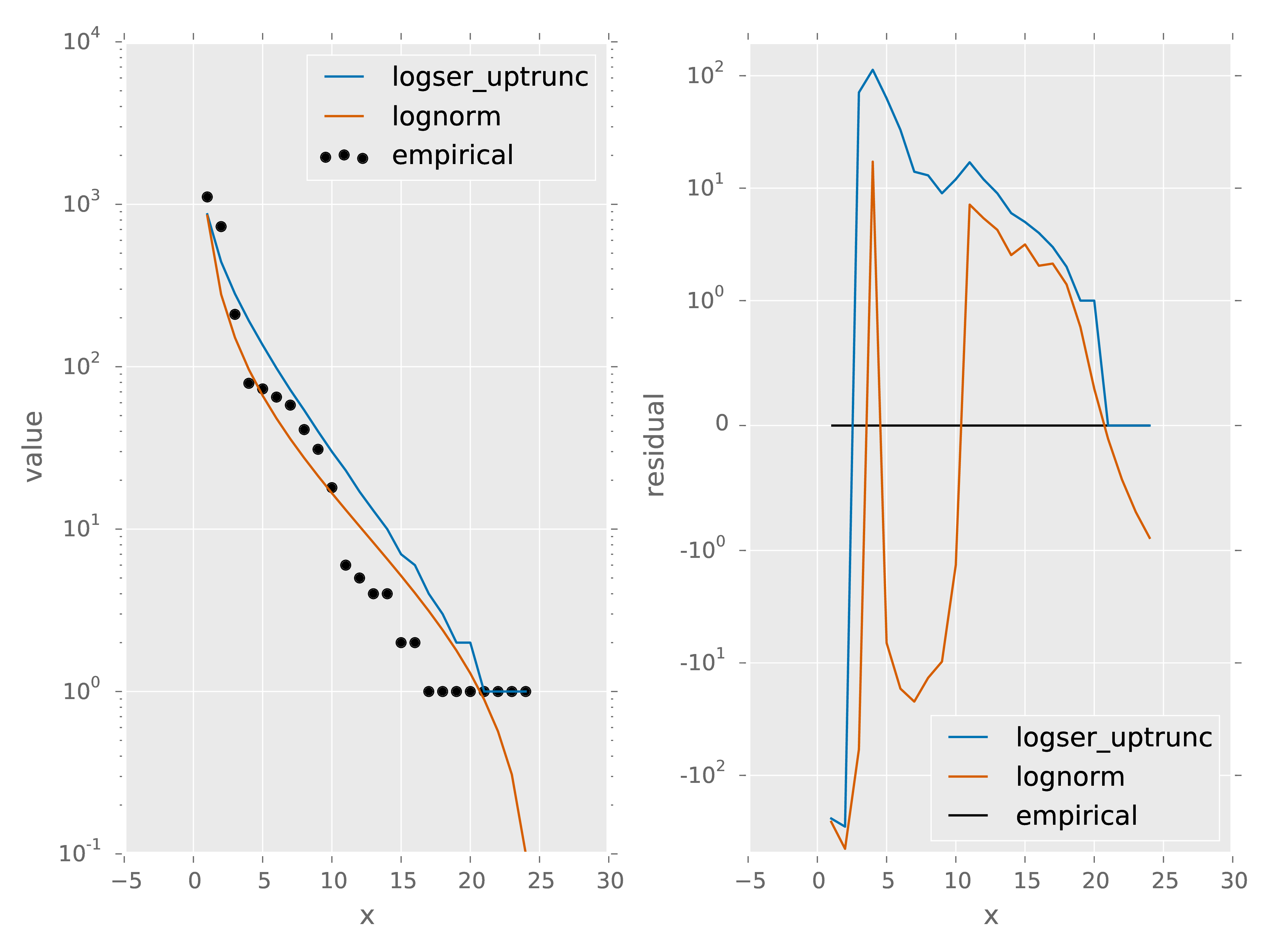
x gives the rank of each species abundance with the most abundance species having a rank of 1. spp gives the species names, empirical gives the empirical species abundance distribution. logser_uptrunc gives the rank abundance distribution predicted by the best fit logser_uptrunc to the empirical data. logser_uptrunc_residual gives the residuals defined as empirical - logser_uptrunc. lognorm and lognorm_residul are defined similarly.
- 1_data_models.pdf: A plot of the information provided in 1_data_models.csv
1_fitted_params.csv: The fitted parameters for models = logser_uptrunc; lognorm to the empirical species abundance distribution for split 1. A description of the different models and their parameters can be found at Models (macroeco.models)
Model Fit Parameters logser_uptrunc 0.9985394369365049 2445.0 lognorm 2.2268165055360067 2.2188336108431264 1_test_statistics: The AIC values (corrected AIC by default) for comparing the goodness of fit of the models specified in models = logser_uptrunc; lognorm to the empirical species abundance distribution for split 1.
Model AIC logser_uptrunc 208.61902087 lognorm 217.82289264